HopPics : Python Implementation of Binary Hopfield Network for self-reconstructing binary images

Github Repository

Installation

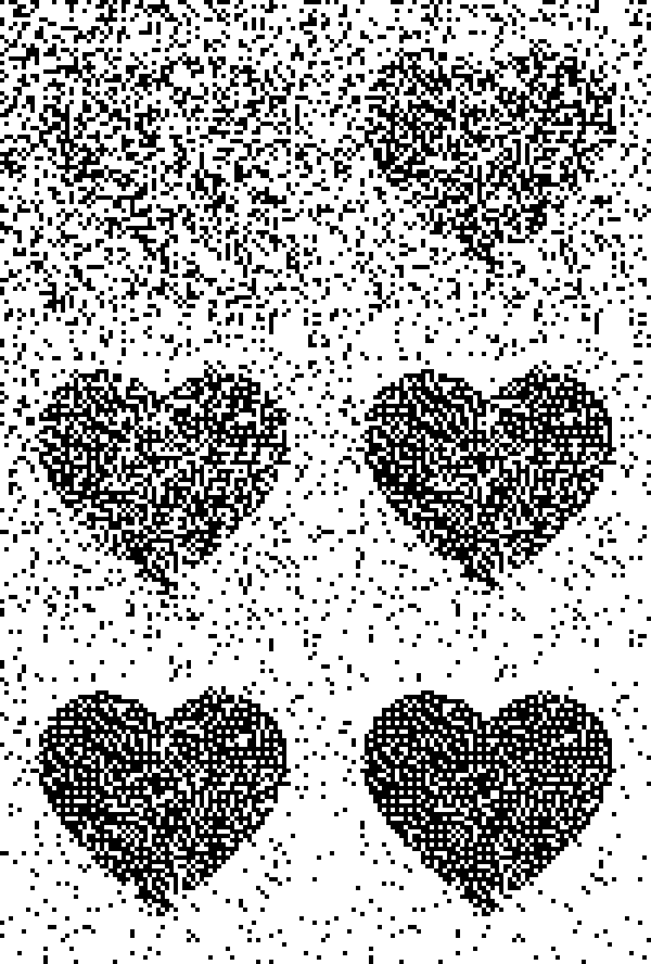
Installing requirements :

$ py -m pip install -r requirements.txt

Usage

Running tests :

$ py test.py <image_path> <nsteps>
$ py test.py example.png 4

Usage in code :

from HopPics import *

hp = HopPics('path_to_pic.png')
hp.reconstruct_from_noise()

I. Introduction

Hopfield networks (HNs) are among the simplest neural networks models. That is because there's almost nothing "neural" about them as they are based on the Ising Model from statistical physics. It only requires basic understanding of matrices and graph theory. It is rather useless in practice but tackles the notion of associative memory and shows a few limitations that are worth taking note of.

This project is a simple implementation of Binary Hopfield Networks to make images that are able to repair themselves through pattern recognition.

II. How it works

A. The Ising Model

As stated before, Hopfield Networks are actually based on Ising models that are normally used in statistiscal physics and the only things that makes it neural is the usage of Hebb's rule which we will see more in detail in the A.

One of the interesting and instrumental concept of the Ising model is the energy function represented by the hamiltonian ie. the total energy of the system :

$$ H = -\sum_{< i,j >} w_{ij} b_i b_j - \mu \sum_{j}h_j bj $$

Where $w_{ij}$ is the interaction between elements i and j of the system and $b_x \in {-1, 1} $ is the state of a node $x$, $\mu$ the magnetic moment and $h_j$ represents the influence of an external magnetic field that we will discard for simplicity or use as a bias.

Our goal with that energy function is to create a system such that :

• The system always converges to a low energy state.
• The system lowers the energy for states that it seeks to remember.

By having these two properties, we will be able to store and retrieve patterns as we'll see in the next part.

B. Training

$$ K = (B,W) $$

Usually Ising models are represented as n-lattices, but in the case of Hopfield Networks, we choose to represent our model as a complete graph K that consists in a set of weights $W$ and a set of nodes $B$. Each node $i \in B$ represents a bit that can either hold the value -1 or 1 and the weights are calculated through a training method which is the Hebbian rule ("Neurons that fire together, wire together"). It is observed that in the brain, when a post-synaptic neuron fires in a small time-frame before the post-synaptic neurons fires, connections between the neurons tend to strengthen. The connection also weakens when the pre-synaptic is firing late compared to it's post-synaptic neuron. Although we don't exactly reproduce this phenomenom in classic HNs since it's a continuous phenomenom and our HNs evolve in discrete time, this concept still allows to create something useful (See this article for more details).

Here is the learning formula that models this phenomenom :

$$ w_{i,j} = {1 \over |B|} \sum_{ p \in P } b_i^p b_j^p $$

Where $w_{ij}$ is the weight of the edge that connects the nodes $i$ and $j$, $P$ is the set of patterns that we wish to train the network to recognize, $b_i^p$ is the value of the node $i$ in the pattern $p$ where in our case $b_i^p \in \{1,-1\}$ and finally $|B|$ is the order of our graph (number of nodes).

What this does is basically making the weights decrease if $b_i^p \ne b_j^p$ because if $b_i^p, b_j^p \in \{1,-1\}$ then $b_i^p * b_j^p = -1 * 1 = -1$. And if they are equal (firing together) then $b_i^p * b_j^p = (-1 * -1) \text{ or } (1 * 1) = 1$. So the weights are "strenghtened" in the case that two neurons are firing at the same time.

C. Associative memory

To calculate each step, we do the following calculations.

$$ b_i = \sum_{j \in B, j \ne i} b_j w_{i,j} $$

And then, each bit goes through an activation function that I chose to be :

$$ \phi(b_i) = sgn(b_i) $$

The fact that the weights are strenghtened if they have the same state will give us what we can call associative memory or pattern recognition. This is because the result of each multiplication between the weight $w_{i,j}$ and the value of each bit $b_j$ in the weighted sum above can pull the value of $b_i$ either towards 1 or -1, and if enough bits $b_j$ in this weighted sum match the trained pattern $b_j^p$ it will be pulled towards $b_i^p$ because of the way we trained our network in II.A. . In that case, the states converge to a low energy state.

III. Examples

Fig 2 : Examples of a destroyed picture of Margaret Hamilton reconstructed after 4 steps.

Fig 3 : Examples of a destroyed image of a panda reconstructed after 8 steps.

Both of these examples have been achieved by first destroying the image by adding random noise to the image (if you squint hard enough you can still see the panda). And even though those image are almost unrecognizable they are still able to snap back to the original if enough pixels are intact.

IV. Conclusion

Hopfield Networks are a great entry point to learning AI and even though HNs are old they might still be useful and interesting to study. More precisely the limitations of HNs are the ones that are worth taking note of as it extends to other models of NNs as well and can help designing other models given a set of constraints and requirements.

For instance, the main limitation of HNs is the limited number of patterns that can be trained for the same model. But another limitation is the possibility for the network to settle for a pattern $p$ that hasn't been trained ($p \notin P$). Also the fact that HNs are recurrent means that they offer little possibility of parallelization.

Recent work has shown that this behaviour of pattern recognition and self-reconstruction can also be achieved through the more convenient method of training cellular automatas to self regenerate or self classification. And I think this is where I'll be headed towards for my next AI project.

Bibliography

• Hopfield Network, Alice Julien-Laferriere
• Hopfield network, John J. Hopfield, Scholarpedia
• Randazzo, et al., "Self-classifying MNIST Digits", Distill, 2020.
• Mordvintsev, et al., "Growing Neural Cellular Automata", Distill, 2020.
• "Neuronal Dynamics From single neurons to networks and models of cognition and beyond", Wulfram Gerstner, Werner M. Kistler, Richard Naud and Liam Paninski